








Customer churn, also known as customer attrition, occurs when a customer stops doing business with a company. In subscription-based industries like software-as-a-service (SaaS), telecommunications, banking, insurance, and media streaming, churn is a critical metric.
A customer who cancels a subscription, switches to a competitor, or simply stops purchasing represents lost future revenue and often higher acquisition costs to replace them.
Churn can be voluntary, the customer actively decides to leave, or involuntary, such as when a credit card expires and the customer does not update payment information.
Voluntary churn includes customers who find a better price, experience poor service, no longer need the product, or feel neglected. Involuntary churn requires different prevention tactics, but both types cost money.
The Financial Impact of Churn
Reducing churn by just five percent can increase profits by twenty five to ninety five percent, depending on the industry.
Acquiring a new customer costs five to seven times more than retaining an existing one. Existing customers also spend more over time. Loyal customers buy additional products, accept upgrades, and refer others.
When a customer churns, the company loses not only the current recurring revenue but also the lifetime value of future purchases.
Despite these facts, many companies react to churn only after it happens. A customer calls to cancel. The retention team offers a discount or a free month.
Sometimes it works, but often the customer has already decided. Reactive retention is expensive and less effective than proactive intervention.
Predictive Churn Prevention
Data mining flips the model from reactive to proactive. Instead of waiting for cancellation calls, data mining algorithms analyze historical customer behavior to identify patterns that precede churn.
A customer who used to log in daily but has not logged in for two weeks. A customer whose support ticket volume spiked last month and then dropped to zero.
A customer who reduced usage from one thousand API calls per day to fifty. Each of these behaviors, in isolation, might be innocent.
But when combined and weighted, they form a churn risk score. With a churn prediction model, a company can intervene before the customer decides to leave.
A high-risk customer might receive a personalized email, a call from customer success, or an automated offer for a feature they have not tried.
The intervention happens while the customer is still engaged enough to notice and respond.
What Data Mining Brings to Churn Prediction
Data mining is the process of discovering patterns in large datasets using methods at the intersection of statistics, machine learning, and database systems.
For churn prediction, data mining algorithms sift through millions of customer records, transaction logs, support interactions, and usage telemetry.
They identify which variables, such as tenure, frequency of login, number of support tickets, average bill amount, payment method, and geographic region, correlate most strongly with churn.
Unlike simple rules like “customers who call support three times churn,” data mining models capture complex interactions.
A customer who calls support twice and has low usage might be at low risk, but a customer who calls support twice and has high usage might be at very high risk.
The model learns these nonlinear relationships from data, not from human intuition.
The Business Value of Churn Prediction
Organizations that deploy data mining for churn prediction see concrete returns. A telecom provider reduced churn by twenty percent by identifying at-risk customers three weeks before they canceled.
A SaaS company increased retention by fifteen percent by automating personalized offers to high-risk users. A bank reduced checking account closures by thirty percent by proactively reaching out to customers whose transaction patterns shifted.
Predicting churn is not about preventing every departure. Some customers will leave regardless of offers.
But focusing retention resources on the customers most likely to churn, and most valuable to retain, maximizes return on retention spending.
Data Sources for Churn Prediction
Raw customer data is rarely ready for mining. Transaction logs contain missing values, inconsistent formats, and irrelevant fields.
Payment histories may be stored in separate tables from usage logs. Support tickets are often unstructured text. Before any churn prediction algorithm can run, data must be extracted, cleaned, transformed, and combined.
This process, called data preparation, typically consumes sixty to eighty percent of the time in a churn prediction project.
The most critical step within preparation is feature engineering, creating the variables that actually predict churn.
Churn models consume data from multiple systems. The CRM provides customer tenure, contract type, billing cycle, payment method, and customer segment.
The product usage database tracks login frequency, feature adoption, API calls, storage used, or minutes watched.
The support system logs ticket volumes, average response time, resolution time, and sentiment of interactions.
Billing systems record payment history, failed payments, invoice amounts, and discount usage. Marketing automation captures email open rates, click through rates, and campaign responses.
Each source has its own update frequency and data retention policies. A typical churn dataset merges these sources at the customer level, creating one row per customer with columns representing their behavior over a specific time window, usually the last thirty, sixty, or ninety days.
Handling Missing and Noisy Data
Missing values are common. A customer may have no support tickets, making that field null. Some usage data may not have been tracked historically.
Strategies for handling missing data include removal, delete customers with too many missing fields, imputation, fill missing values with medians or zeros, or creating a separate category for “missing” as a meaningful signal.
For example, customers who have never logged a support ticket behave differently from those who have.
Noisy data includes outliers that can skew models. A single customer who made ten thousand API calls in one day due to an automated script may not represent typical usage.
Winsorization caps extreme values at the ninety ninth percentile. Domain knowledge also helps.
If a customer’s reported monthly bill exceeds the maximum plan price, that is likely a data entry error requiring correction.
Feature Engineering for Churn Prediction
Feature engineering is where domain expertise meets data mining. Raw fields like “last login date” become features such as “days since last login” or “login frequency in past thirty days.”
A single date field can generate multiple features: day of week, hour of day, days since first login (tenure), days since most recent login (recency).
Behavioral sequences become aggregated counts: number of support tickets in last seven days, thirty days, and ninety days.
Trend features capture direction: is usage increasing, decreasing, or stable? A customer whose usage dropped fifty percent month over month is different from one with steady usage.
Common churn prediction features include recency, days since last login, last purchase, last support interaction. Frequency includes logins per week, purchases per month, tickets per quarter.
Monetary includes average bill amount, payment delay days, total lifetime value. Engagement includes number of features used, pages viewed per session, session duration.
Support includes tickets submitted, average resolution time, number of escalations. Contract includes contract length, months remaining, auto renewal status.
Payment history includes failed payment attempts, credit card expiration approaching.
Temporal Windows and Observation Points
Churn prediction models require careful temporal alignment. The data used to predict churn must come from a period before the churn event.
A common approach is to define an observation window, such as days one to ninety of a customer’s life, and a prediction window, such as days ninety one to one hundred twenty.
Features are calculated only from the observation window. The target variable, whether the customer churned during the prediction window, is labeled after the fact.
This prevents look ahead bias, where the model inadvertently uses future information to predict the past.
Rolling windows allow models to be updated over time. Instead of a single observation window, features are recomputed every week using the most recent ninety days of data.
The model then predicts churn in the next thirty days. This sliding window approach adapts to changing customer behavior patterns.
Defining Churn
Defining churn is not always simple. For a monthly subscription, churn may be cancellation or failure to pay after a grace period.
For a freemium product, churn might be zero usage for sixty days. For an ecommerce site, churn could be no purchase in twelve months.
The definition must match business reality. A poorly defined target variable, labeling customers as churned when they are merely inactive but still valuable, will produce a model that optimizes for the wrong outcome.
Choosing the Right Algorithm
With clean data and engineered features, the next step is selecting and training a predictive model.
Logistic regression is a classification algorithm that outputs a probability between zero and one. For churn prediction, the probability represents the likelihood that a customer will churn within a defined time window.
The model learns coefficients for each feature. A one day increase in “days since last login” might increase churn probability by two percent.
These coefficients are highly interpretable. Logistic regression works well when relationships between features and churn are roughly linear.
Random forests solve overfitting by building hundreds of decision trees, each trained on a random subset of data and random subset of features.
Random forests are among the most accurate off the shelf algorithms for churn prediction. They handle mixed data types without extensive preprocessing.
Gradient boosting builds trees sequentially, each new tree correcting the errors of the previous ones. Algorithms like XGBoost and LightGBM dominate churn prediction competitions because they deliver state of the art accuracy.
They handle missing data natively, support regularization to prevent overfitting, and train faster than random forests on large datasets.
Evaluation Metrics for Churn Models
Accuracy is misleading for imbalanced churn data. Better metrics include precision, recall, F1 score, and Area Under the ROC Curve.
Precision measures of customers predicted to churn, what fraction actually churned. High precision means few false alarms, saving retention budget.
Recall measures of customers who actually churned, what fraction did the model catch. High recall means fewer missed churners.
F1 score is the harmonic mean of precision and recall. AUC above 0.8 is good; above 0.9 is excellent.
Deploying the Model into Operations
A churn prediction model has no value until it influences customer behavior. Batch deployment runs predictions on a schedule, nightly, weekly, or monthly.
The model scores every active customer, producing a churn probability for each. These scores are written back to the CRM.
Retention teams then query the CRM for customers with scores above a threshold, export the list, and begin outreach.
Real-time deployment embeds the model directly into customer-facing systems. When a customer performs an action, logging in, starting a support chat, viewing a cancellation page, the system calls the model API.
It receives a churn score in milliseconds and triggers an automated response. A customer with a high churn score who lands on the cancellation page might see a pop up offer.
Designing Effective Retention Interventions
The prediction is only half the solution. The intervention must be relevant and cost effective.
Proactive customer success outreach involves a customer success manager calling or emailing high-risk customers to offer assistance. Best for high-value customers.
Automated discount offers can be effective for price sensitive churn but train customers to expect discounts. Should be used sparingly.
Feature education campaigns highlight features the customer has not used. Often effective for engagement driven churn.
A/B Testing and Model Monitoring
Never assume an intervention works. Run controlled A/B tests. Randomly split high-risk customers into a treatment group, receives the intervention, and a control group, receives no intervention.
Compare churn rates between the two groups after thirty or sixty days. The difference is the true lift attributable to the intervention.
Customer behavior evolves. A model trained on data from 2023 may perform poorly in 2025. Models experience concept drift.
Monitor data drift, prediction distribution, and business metrics. Establish a retraining schedule. Monthly retraining is common for fast changing businesses.
Data mining transforms customer churn from a reactive post mortem into a proactive opportunity. Clean data and thoughtful feature engineering feed algorithms like logistic regression, random forests, or gradient boosting.
The resulting model scores every customer with a churn probability. But the real value comes from deployment, batch or real time, and from well designed, A/B tested interventions that actually retain customers.
Ongoing monitoring catches model drift, and retraining keeps predictions accurate. Organizations that close the loop from prediction to action to measurement reduce churn, increase customer lifetime value, and gain a lasting competitive advantage.